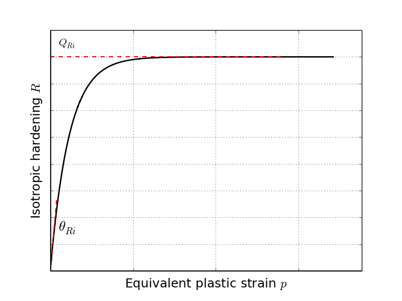
Fig 1: Voce term representation
This tutorial covers the procedure to optimise an isotropic hardening rule to describe the behaviour of a metallic material at large strains.
This tutorial requires:
To obtain a correct isotropic hardening rule at large strain, the methodology uses a numerical/experimental correlation based on trial and error method. The basic idea is to modify some of the parameters obtained by MatPrePost until a good agreement is found with the experimental data.
In the SIMLab Metal Model, the isotropic hardening rule is defined using a 3 term Voce, expressed as:
\(R = \sum_{i=1}^3 Q_{Ri}.\left( 1-e^{\left( -\frac{\theta_{Ri}}{Q_{Ri}}.p\right)}\right)\)
where \(p\) is the equivalent plastic strain, \(\theta_{Ri}\) and \(Q_{Ri}\) are the initial hardening modulus and the saturation stress of the \(i\) Voce term respectively. A graphical illustration of a Voce term is given in Figure 1, where the hardening modulus and saturation stress are depicted. The Voce terms will also saturate with \(Q_{Ri}\) as the asymptote while \(\theta_{Ri}\) will drive the speed at which the saturation will occur.

Fig 1: Voce term representation
As explained in the MatPrePost tutorial "Identification of an isotropic hardening rule from small to intermediate strain", the Voce parameters are only valid up to diffuse necking. Some of these parameters have to be optimised to describe the post necking regime of a tensile test. Usually, 3 Voce term are used to describe the strain-stress curve of a metallic alloy (some alloys or temper may require only one but this is not covered here) leading up to 6 parameters to be modified.
For convenience reasons, it is important to re-order (if not done by MatPrePost) the Voce terms such as: \(\theta_{R1}^0 > \theta_{R2}^0 > \theta_{R3}^0\).
To determine which of the Voce terms has to be modified it possible to plot the isotropic hardening terms \(R_i\) versus the equivalent plastic strain in the same graphic as the engineering stress-strain curve as shown in Figure ??. When using this technique two scenario can arise:

Fig 2: Case scenario 1
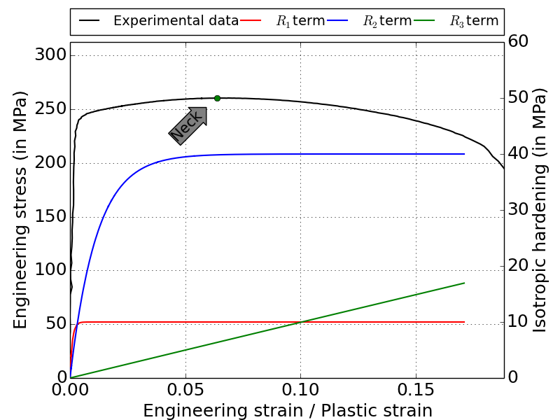
Fig 3: Case scenario 2
Regarding the first Voce term \(R_1\), it is most likely to be saturated before diffuse necking since it is representing the initial knee in the stress-strain curve. With respect to the two case scenario:
For the case scenario 1, a first simulation should be run with all the identified Voce terms. Again, two results can be obtained, the model can overestimate the post necking response (red dashed curve) or underestimate it (blue dashed curve). If the model overestimates the experimental test, either \(\theta_{R3}\) and \(Q_{R3}\) or both have to be modified. To get a better correlation with the test, the parameter \(Q_{R3}\) can be decreased while the hardening modulus \(\theta_{R3}\) should be increased.

Fig 4: First simulation
For the case scenario 2, one simulation with all Voce terms should be run, one with all Voce terms and one without the third Voce term. This will help finding if the third Voce term is necessary in the model. Using the same illustration as before:
Following the item 1, the simulation without the second Voce term should either underestimate or overestimate the experimental data. If the model under predicts the post necking behaviour then the parameters \(\theta_{R3}\) and \(Q_{R3}\) should be modified. On the other hand, if the simulation still overestimate, then the parameters \(\theta_{R2}\) and \(Q_{R2}\) should be modified and the third Voce term should be cancelled.
As a general rule when the \(\theta_{Ri}\) or \(Q_{Ri}\) have to be modified it is suggested to use the following method:
\(X = X .\left( 1\pm \kappa \right)\)
where \(X\) is the parameter to be modified and \(\kappa\) is the perturbation. As a starting point \(\kappa = 0.5\) can be used and increased or decreased depending on the results. As a general recommendation, the user should copy and paste his/her material cards into the same text file to keep track of the evolution of the parameters.
The engineering stress-strain curve of the tensile test should be used to carry out the numerical/experimental correlation. This will allow to damp out the differences due to machining tolerance i.e the width of a tensile specimen could 4.95 mm while the FE model will be 5 mm.
This tutorial relies on the use of an uni-axial tensile test. A 6XXX aluminium alloy in temper T6 with a nominal thicknesss of 2 mm is used here. This alloy is produced by extrusion. An overview of the material is given in Figure 1, the different specimens show a rather low scatter in terms of engineering strains and stresses.
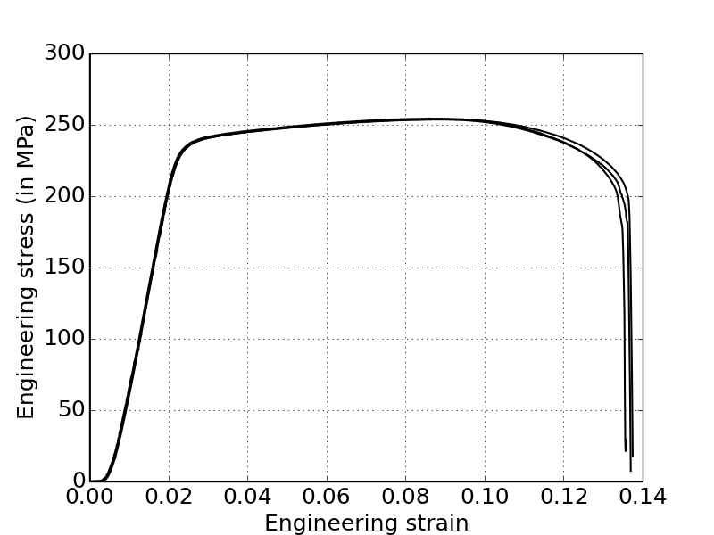
Fig 5: Test replicates
NOTE: The displacement used here to compute the engineering strain is the head cross one,
therefore the reader should not pay attention to the stiffness in the elastic domain.The tensile test specimen is based on the ResOrg database and uses the UT 60 shape (see Figure 2).
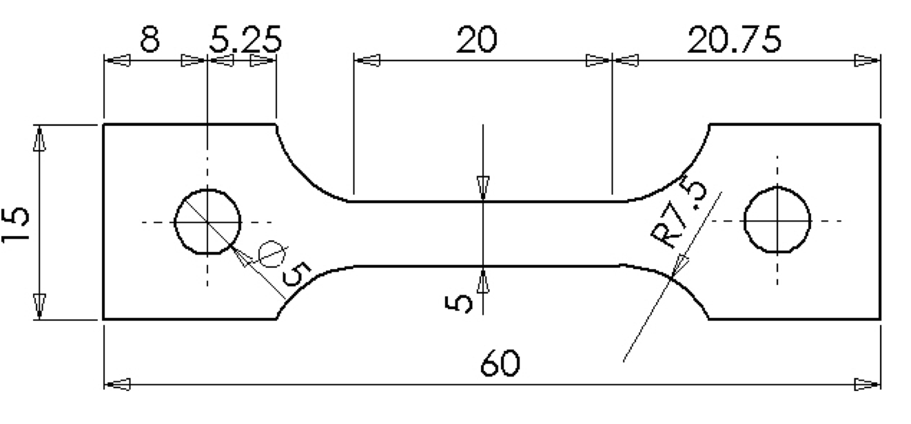
Fig 6: UT 60
In addition to the force measured by the load cell and the displacement of the head cross, DIC measurements were also carried out to extract virtual extensometers. A longitudinal extensometer was extracted on a length of 8.2 mm over the neck in the selected tensile specimen.
The tensile test is simulated using a solid element mesh as shown in Figure 3. One symmetry plane through the thickness is applied resulting into a 5 solid elements representing half of the thickness. The FE model incorporates a total of approx. 20 000 solid elements with a reduced integration scheme.

Fig 7: Finite element model
The specimen is loaded through rigid pins, their diameter is slightly smaller than the holes to remove potential initial contact problems. The implicit solver of ABAQUS is used in this tutorial to run the described FE model. The optimum number of cpus is 8 for this model, leading to a computational time of approx. 5 min.
The SIMLab Metal Model is set up for this application to the following choices:
The material resulting from these choices should be set up like:
| 1 | 2 | 3 | 4 | 5 | 6 | 7 | 8 |
|---|---|---|---|---|---|---|---|
| EFLAG | YFLAG | RMAPFLAG | HFLAG | VFLAG | TFLAG | DFLAG | SFFLAG |
| STFLAG | \(E_0\) | \(\nu\) | \(\sigma_0\) | \(\xi\) | \(\theta_{R1}^0\) | \(Q_{R1}^0\) | \(\theta_{R2}^0\) |
| \(Q_{R2}^0\) | \(\theta_{R3}^0\) | \(Q_{R3}^0\) |
where EFLAG = 1, YFLAG = 1, RMAPFLAG = 4, HFLAG = 1 and the remaining flags are equal to zero.
By applying the MatPrePost tutorial dealing with isotropic hardening for small and moderate strains, the user should obtain a first set of parameters describing the yielding and hardening of the considered material. Using MatPrePost, the following parameters are found (here expressed in MPa).
| \(\sigma_0\) | \(\theta_{R1}^0\) | \(Q_{R1}^0\) | \(\theta_{R2}^0\) | \(Q_{R2}^0\) | \(\theta_{R3}^0\) | \(Q_{R3}^0\) |
|---|---|---|---|---|---|---|
| 223.9 | 20266.0 | 15.9 | 1953.8 | 3.9 | 904.3 | 52.09 |
NOTE: The user may not find the exact same parameters as mentioned here since the selection of the yield point is
     determining the fitting of the hardening parameters.
To determine which of the hardening parameters needs to be modified, a simple visualisation of the engineering stress-strain curve versus the different hardening terms (\(R_i\)) can be used. The following pictures illustrates the above mentioned data for the current material.
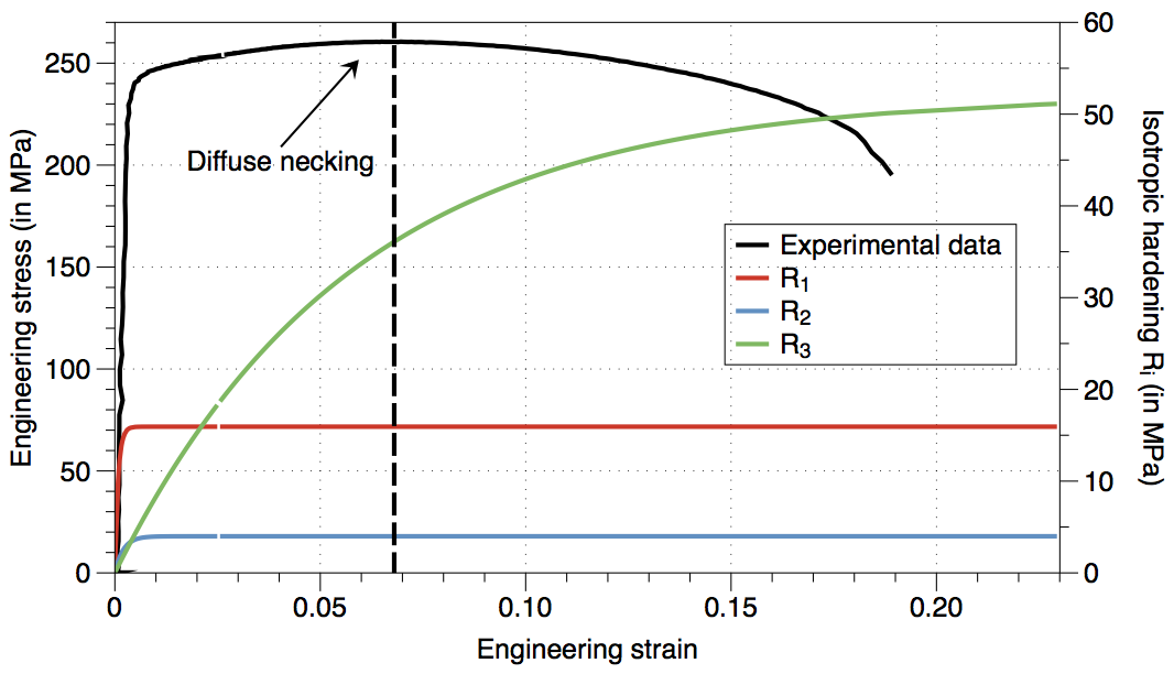
Fig 8: Isotropic hardening terms
From this figure, it can be seen that the third Voce term \(R_3\) is the only one which is not saturated after diffuse necking. As the \(R_1\) and \(R_2\) are completely saturated before that point they won't have any impact on the post necking behaviour. The optimisation of the hardening parameters should therefore be focused on the \(\theta_{R3}^0\) and \(Q_{R3}^0\).
To determined how the \(\theta_{R3}^0\) and \(Q_{R3}^0\) parameters shall be modified the first step is to run an analysis using the parameters found by MatPrePost. Figure ??, shows the results in terms of engineering stress and strain obtained with the MatPrePost fitted parameters.
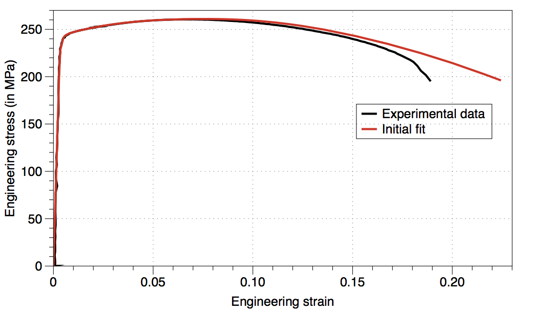
Fig 9: Initial parameters
First of all, the initial fit from MatPrePost shows a very good correlation up to diffuse necking as expected. There is a slight overshoot of the stress-strain curve after necking. This indicates that the saturation stress \(Q_{R3}^0\) should be decreased. By setting \(Q_{R3}^0\) equal to 49 MPa instead of 52 MPa as identified the agreement is found to be satisfying.
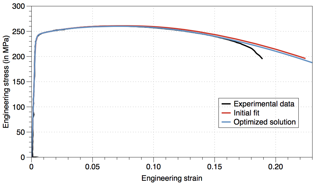
Fig 10: Optimised parameters
Please visit http://google.com/ for other tutorials.
© 2014 SIMLab-SINTEF-NTNU. All rights Reserved.